18 Jan Multi-Layered Perceptron
 Multi-Layered Perceptron
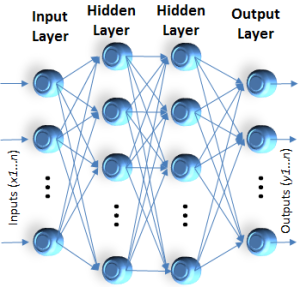
In prior posts we introduced the concept of the artificial neural network and the perceptron model as a simple implementation of a neural network. We showed the structure, including an input layer and an output layer. Let’s look at one of the typical approaches for processing input to derive the output. The net output of each layer determines the input of the next.
The net output formula is intended to mimic the flow of excitation and inhibition through layers of the brain, affecting many neurons from beginning to end. This illustration shows that the final output y is the vector of weights derived from the last layer of neurodes based on the incoming weights. The layers between input and output are described as “hidden” because their values are not independently meaningful, even though they contribute to the final output.
| Understanding Context Cross-Reference |
|---|
| Click on these Links to other posts and glossary/bibliography references |
|
|
|
| Prior Post | Next Post |
| Learning from Errors | |
Definitions |
References |
| Feldman 1982 | |
| Anderson 1988 | |
| Rosenblatt 1958 |
 Winner Takes All
The formula for calculating the output of a multi-layered perceptron can also be stated as a matrix operation in which the input matrix and the weights are combined to yield an output b. A set of m patterns X of length n will yield a set of outputs b. Weights are multiplied with input to determine each layer’s output. The output is then fed as input into the formula for determining the next layer’s value. Threshold values can be set to produce output only if the input value is high enough.
In connectionist networks similar to that in the figure on the previous page, input patterns (strings of 1s and 0s) are fed to the first layer of PEs. Each connection from each processor has a weight, often between -1 and 1, stepping in 10ths or 100ths. Prior to “learning,” weights are random or arbitrary. As each input is repeatedly fed into the network, the weights are gradually adjusted, automatically, according to positive and negative feedback. The network then becomes able to recognize inputs – that is, the network will yield a certain pattern of output each time it encounters the same input. The pattern yielded may be a pattern of active PEs in the net or the output layer, or the pattern may be a single fired or hyperactivated PE. Many ANS use a winner-take-all (WTA) procedure to interpret output. The WTA formula is shown on the next page.
 The winner-take-all model described above has two important meanings in our attempt to imitate what we think is happening in the brain:
- individual processes, such as recognition, will yield a result (either succeed or fail to recognize input x); and
- collective processes, such as decision making, will have a result.
The collective processes are more likely to require conscious weighing of the options.
You’re Fired
An important part of understanding ANS responses to input is the winner-take-all concept. Between each input, all PEs rest with a zero value. On receiving input, the output of the network shows whether it “recognizes” the pattern or not. Feldman & Ballard describe it this way: “One way to deal with the issues of coherent decisions in a connectionist framework is to introduce winner-take-all (WTA) networks, which have the property that only the unit with the highest potential (among a set of contenders) will have output above zero after some setting time” (1982, p.226).
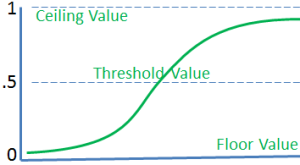
WTA can be implemented using a threshold value between zero and the maximum value, then firing all PEs that receive input equal to or greater than the threshold value. A fired PE changes from zero to one. The functions shown in the illustration at left depict the square stepping function (blue) and the smoother sigmoidal curve (purple) of threshold logic. The sigmoidal function tends to be preferred in many ANS, possibly because of its symmetry with activation patterns in the human brain. The values shown are between 0 and 1 with a threshold at .5, but the values can be set arbitrarily.
 A sigmoidal activation function for WTA shows that it is a threshold function. In this case, the threshold is 0.5. The similarities with the curve of synaptic firing through the aggregate impact of received impulses of excitation and inhibition is not accidental, though it is not a perfect match.
Although the formula produces a sigmoidal curve, WTA squares it by making all results below the threshold not fire and all results above the threshold fire.
| Click below to look in each Understanding Context section |
|---|


