05 May Learning from Errors

If at first you don’t succeed, try – try again. Humans are pretty good at learning from our mistakes. In fact, some suggest that whatever doesn’t kill you makes you stronger. Today I’d like to riff on that theme a bit, and talk about ways in which machines can implement learning from errors.

Error Minimization

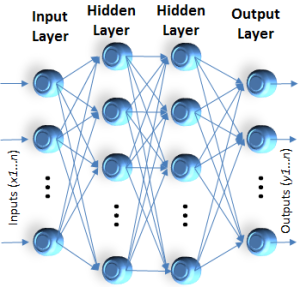
One of the amazing advances of neural networks is their ability to learn through repetition. You tell them what the pattern means by explaining the correct output for a given input, and the neural network will adjust its weights in the arcs between nodes until it can consistently deliver the correct output. The formula for learning in a connectionist network was suggested earlier in the reference to Duda and Hart’s work in pattern classification. Learning can be implemented as a process of error minimization. The appeal of this approach in a distributed environment is that local error minimization on the individual neurodes and weights can have a global effect. In fact, this property is probably the major advantage of ANS for perception-related processing. A stimulus is received (a vector is input), and the network feeds it through its layers over weighted arcs. The threshold logic determines the output. Prior to learning, the output will be in error most of the time, but because the actual output can be compared with the desired output, the error e can be calculated.

Understanding Context Cross-Reference
Click on these Links to other posts and glossary/bibliography references

Section 3 #18

Table of Context

Prior Post	Next Post
Multi-Layered Perceptron	Impulse Waves in Layers
Definitions	References
learning neural network	Duda 1973 SRI Algorithm
input classification output	SRI Work Anderson 1988
connectionism ANS neurodes	Rosenblatt 1958

Adult learning can often be done through internal or self-correction. We observe that our actions or words do not achieve the desired outcome, so we try something else. For children who have not yet developed the advanced powers of observation and correlation, supervised learning is needed. Someone who knows corrects them. Computers are like little kids – needing constant reinforcement in learning.

Calculated error can be used as the basis for adjusting weights locally to produce the desired output. Because the system is intended to deal with many patterns, rather than forcing the system to the correct output for a single input immediately, weights are adjusted slowly to converge on the correct output. This means that learning requires many cyclic iterations of each input to converge on recognition, but it does enable the learning of many patterns.

Generalized Delta Rule

A widely used adaptation formula for adjusting weights to converge is called the generalized delta rule, which is shown with the error calculation formula below. The formulae are straightforward. The delta rule is particularly eloquent in its ability, when applied to a distributed network of neurodes with weighted links, to simulate learning and yield a robust, fault-tolerant computing mechanism. Fault-tolerance, in this context, is a function of two things:

the network’s ability to recognize patterns despite the presence of noise; and
the ability of the network to continue to function despite the failure of some of the neurodes or links in the physical structure.

On initial input, the output weights will be incorrect. Where “targ” is the target value of output l given pattern k, the following formula calculates the error:

Propagating change formulae back through the network can be a basis for changing weights and permitting the network to learn.

The formula below is the generalized delta rule in which the weights W from neurodes n can be calculated.

An algorithm that uses errors in the output (discreet differences between the correct output and the actual output) to train an artificial neural system to derive a correct output automatically.

Here’s an excerpt from Stanford Research Institute International site explaining a common algorithm for training neural networks:

A Backpropagation Algorithm

1.

Propagates inputsforward in the usual way,i.e.

All outputs are computed using sigmoid thresholding of the inner product of the corresponding weight and input vectors.
All outputs at stage n are connected to all the inputs at stage n+1

2.

Propagates the errors backwards by apportioning them to each unit according to the amount of this error the unit is responsible for.

We now derive the stochastic Backpropagation algorithm for the general case. The derivation is simple, but unfortunately the book-keeping is a little messy.

$\vec{x_j} =$ input vector for unit j (x_ji = ith input to the jth unit)
$\vec{w_j} =$ weight vector for unit j (w_ji = weight on x_ji)
$z_j = \vec{w_j}\cdot \vec{x_j}$ , the weighted sum of inputs for unit j
o_j = output of unit j ( $o_j = \sigma(z_j)$ )
t_j = target for unit j
Downstream (j) = set of units whose immediate inputs include the output of j
Outputs = set of output units in the final layer

Since we update after each training example, we can simplify the notation somewhat by imagining that the training set consists of exactly one example and so the error can simply be denoted by E.

We want to calculate $\frac{\partial E}{\partial w_{ji}}$ for each input weight w_ji for each output unit j. Note first that since z_j is a function of w_ji regardless of where in the network unit j is located,

$\begin{eqnarray*}\frac{\partial E}{\partial w_{ji}} &=& \frac{\partial E}{\parti... ...rtial w_{ji}} \\ &=& \frac{\partial E}{\partial z_j} x_{ji}\\ \end{eqnarray*}$

Furthermore, $\frac{\partial E}{\partial z_j}$ is the same regardless of which input weight of unit j we are trying to update. So we denote this quantity by $\delta_j$ .

Consider the case when $j \in Outputs$ . We know

$\begin{displaymath}E = \frac{1}{2}\sum_{k \in Outputs} (t_k - \sigma(z_k))^2 \end{displaymath}$

Since the outputs of all units $k \ne j$ are independent of w_ji, we can drop the summation and consider just the contribution to E by j.

$\begin{eqnarray*}\delta_j = \frac{\partial E}{\partial z_j} &=& \frac{\partial }... ...o_j)(1-\sigma(z_j))\sigma(z_j)\\ &=& -(t_j - o_j)(1-o_j)o_j\\ \end{eqnarray*}$

Thus

$\begin{displaymath} \Delta w_{ji} = -\eta \frac{\partial E}{\partial w_ij} = \eta \delta_j x_{ji} \end{displaymath}$

Now consider the case when j is a hidden unit. Like before, we make the following two important observations.

1.: For each unit k downstream from j, z_k is a function of z_j
2.: The contribution to error by all units $l \ne j$ in the same layer as j is independent of w_ji

We want to calculate $\frac{\partial E}{\partial w_{ji}}$ for each input weight w_ji for each hidden unit j. Note that w_ji influences just z_j which influences o_j which influences $z_k \forall k \in Downstream(j)$ each of which influence E. So we can write

$\begin{eqnarray*}\frac{\partial E}{\partial w_{ji}} &=& \sum_{k \in Downstream(j... ...al o_j} \cdot \frac{\partial o_j}{\partial z_j} \cdot x_{ji}\\ \end{eqnarray*}$

Again note that all the terms except x_ji in the above product are the same regardless of which input weight of unit j we are trying to update. Like before, we denote this common quantity by $\delta_j$ . Also note that $\frac{\partial E}{\partial z_k} = \delta_k$ , $\frac{\partial z_k}{\partial o_j} = w_{kj}$ and $\frac{\partial o_j}{\partial z_j} = o_j (1-o_j)$ . Substituting,

$\begin{eqnarray*}\delta_j &=& \sum_{k \in Downstream(j)} \frac{\partial E}{\par... ... &=& \sum_{k \in Downstream(j)} \delta_k w_{kj} o_j (1-o_j)\\ \end{eqnarray*}$

Thus,

$\begin{displaymath} \delta_k = o_j (1-o_j) \sum_{k \in Downstream(j)} \delta_k w_{kj} \end{displaymath}$

We are now in a position to state the Backpropagation algorithm formally.

Formal statement of the algorithm:

Stochastic Backpropagation (training examples, $\eta$ , n_i, n_h, n_o)

Each training example is of the form $\langle \vec{x}, \vec{t} \rangle$ where $\vec{x}$ is the input vector and $\vec{t}$ is the target vector. $\eta$ is the learning rate (e.g., .05). n_i, n_h and n_o are the number of input, hidden and output nodes respectively. Input from unit i to unit j is denoted x_ji and its weight is denoted by w_ji.

Create a feed-forward network with n_i inputs, n_h hidden units, and n_o output units.
Initialize all the weights to small random values (e.g., between -.05 and .05)
Untilterminationconditionis met, Do
- For each training example $\langle \vec{x}, \vec{t} \rangle$ , Do

1. Input the instance $\vec{x}$ and compute the output o_u of every unit.
2. For each output unit k, calculate: $\begin{displaymath}\delta_k = o_k(1-o_k)(t_k - o_k) \end{displaymath}$
3. For each hidden unit h, calculate: $\begin{displaymath}\delta_h = o_h(1-o_h)\sum_{k \in Downstream(h)} w_{kh}\delta_k \end{displaymath}$
4. Update each network weight w_ji as follows:

$\begin{eqnarray*}w_{ji} &\leftarrow& w_{ji} + \Delta w_{ji}\\ {\rm where} \quad \Delta w_{ji} &=& \eta \delta_j x_ji\\ \end{eqnarray*}$

For perceptual tasks such as vision (object recognition) and speech recognition, this model works beautifully. It is well suited for many two-dimensional tasks including trend analysis, where the trend can be defined in two-dimensional terms such as trend-line graphs. We will return to this model whenever we encounter tasks of this nature, and effectively use artificial neural networks with learning algorithms such as back propagation.

Click below to look in each Understanding Context section

Intro	Context	1	Brains	2	Neurons	3	Neural Networks
4	Perception and Cognition	5	Fuzzy Logic	6	Language and Dialog	7	Cybernetic Models
8	Apps and Processes	9	The End of Code		Glossary		Bibliography

Posted by Joe Roushar in Cognitive Science, Communication, Knowledge, Learning, Memory, Neural Networks, Neuroscience, Ontology , Followed with Comments Off

Post Tagged with Backpropagation, cognitive modeling, context, cybernetics, fuzzy logic, information, intelligence, interpretation, knowledge, learning, Learning from Errors, neural network, Neuromorphic Computing, understanding

SHARE THIS ARTICLE

Comments are closed.

Recent Posts

Recent Comments

05 May Learning from Errors

Error Minimization

Generalized Delta Rule

A Backpropagation Algorithm

SHARE THIS ARTICLE