24 Jul Pattern Classification in Space
Pattern Classification
 Visual patterns can be recognized and classified based on prior knowledge: I see that this hairy animal has four legs and is about the same size as my dog, so I’ll assume it is (or classify it as) a dog. This may not be a correct classification, but it’s more correct than classifying it as an airplane, house or person. If we’d never seen anything like a dog before, we would have no basis for classifying it. In this case, the statistical likelihood of successful classification is nil – worse than playing slot machines or roulette.
Classification can be treated as a statistical decision process intended to minimize error or minimize the probability of wrong decisions. In the real world, there is a correlation between wrong decisions and unnecessary costs, so the decision process can be treated as a cost calculation. The beauty of pattern classification is that, except in novel cases in which the pattern encountered is completely unique, you can compare it with similar or exactly matching stored patterns. Hopefully, the statistical probability of correct classification is better than the probability of winning at slots or roulette.
| Understanding Context Cross-Reference |
|---|
| Click on these Links to other posts and glossary/bibliography references |
|
|
|
| Prior Post | Next Post |
| Parallel Distributed Pattern Processing | |
Definitions |
References |
| Duda 1973 | |
| Hebb 1949 | |
| Selfridge 1958 |
In order to facilitate the process of making decisions, it is best to break the problem down into component parts based on the nature of the factors (or constraints) that go into the decision. Each factor has underlying information that I have been calling features, and breaking these features down into categories makes it easier to spot and act on patterns in the information. As Duda and Hart put it, “The problem of classification is basically one of partitioning the feature space into regions, one region for each category. Ideally, one would like to arrange this partitioning so that none of the decisions is ever wrong” (1973, p.5).
Feature Types
 Feature spaces can be one, two, three or multi-dimensional spaces in which decision constraint types, such as “textual”, “graphical”, Numeric”, etc., divide the probable characteristics of the classes of patterns required.
A number or other character string has a single dimension: length. We match the string from left to right, even though it may be displayed vertically for human consumption as in some Asian languages. The exact number or string may be matched, or a fuzzy matching algorithm may yield near matches. In one-dimensional matching, the sequence of characters is the most important characteristic of the pattern. An implicit characteristic of one-dimensional matching is the frequency of recurrence or individual elements. One may extend the sequence model to match any pair of adjacent characters. One may relax the model further by establishing proximity rules, not requiring input pattern elements to be direct neighbors even if they are in the stored pattern. I will further explain the importance of adjacency and proximity as I post on language understanding algorithms.
Images are two-dimensional. Sequence, proximity and adjacency, as well as line, angle, color, curve, light and dark and other characteristics define image patterns. Using height (x) and width (y) axes, every pixel of an image can be compared with other images. Image comparison algorithms, especially for facial recognition, have become important in social media and law enforcement.
3-D images add a depth dimension to further complexify pattern matching, but can be easily flattened out to two dimensions. This may be what we do in our visual interpretation process. Videos are always three-dimensional because they add the dimension of time, specifically change over time, to the dimensions of height and width.
If we don’t specify the constraint type in advance, we need a real-time mechanism for scanning the data and ensuring that it is an appropriate data type otherwise the pattern match is likely to fail. Once we have a pattern to match against a set of patterns in memory, we can assign the appropriate heuristic for that data (constraint) type. Probabilities of a match, in this framework, are described as a priori, joint, conditional, and a posteriori, and are the basis for partitioning feature space in deterministic processes.
Artificial Neural Systems (ANS)
Spatial distribution of patterns according to probabilities is analogous to techniques used non-deterministically in ANS; probability theory was one of the main catalysts in the invention of mathematical approaches to pattern recognition. The concept of a distributed feature space for decision making and a distributed computational space for representing the data, and possibly even learning to classify patterns, is intuitively very appealing.
Here is an example of categories of information that could go into a decision. If MIPUS must decide whether or not to clear the table, he must observe levels, functions and commands.
- A command to “Clear the Table” would be sufficient to begin.
- A content or descriptive level observation of “No food remaining on any plate” would be sufficient to begin.
- A functional observation of “No person eating any food” would be sufficient to begin.
Filtering and Sorting Patterns
 Above, I used the phrase “patterns in the information” because many pattern classification problems involve selecting some information from among multiple different patterns, and filtering out the rest. An example is the problem of facial recognition. I am meeting my friend downtown, and I know he’ll be walking down a specific sidewalk. I can see buildings, automobiles, parking meters, trees, and many people. I have placed an image of my friend at the front of my mind (whatever that means) and I’m looking for a match
Linear Discrimination
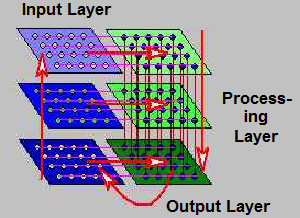
Pattern classification by linear discrimination can be performed by complex multi-layered networks as well as by using the perceptron model. An example of a multi-layered linear discriminator is shown in the illustration below. Adjusting weights of links or “synapses” as a model of learning was proposed as early as the late 1940’s (Hebb, 1949) and was elucidated in terms more suitable for designing automatic learning mechanisms by Selfridge and others a decade later in the application domain of learning to interpret Morse code.
 In a multi-layered network model, a layer of PEs (demons) was linked to a second layer of PEs (subdemons), and interaction with the environment governed the evolution of a capability to correctly interpret code. The interactions were limited to positive (correct) examples of input and, after the machine responded to the input, positive or negative reinforcement (Selfridge, 1958). Subsequent models have incorporated negative input examples as well. The formula for a multi-layered perceptron matrix operation is shown below:
Before we get too muddled in the mathematics of linear discrimination, let’s remind ourselves of what we are trying to do. Neurons in the brain receive impulses (input) of varying levels and send or propagate impulses (output) of varying levels. This mechanical process is the basis of all cognitive processes. Recognizing input, whether visual, auditory or other input, requires discrimination. The perceptron model is a way to recognize input.
Neural networks and perceptrons have proven very powerful in recognizing characters in written languages, images, and trend lines. These are all two-dimensional problems. Once a third dimension is added, neural network discrimination tends to weaken or completely collapse. In the upcoming posts, I will show other options for processing multi-dimensional patterns.
| Click below to look in each Understanding Context section |
|---|


